Demodulation and Measurement
The demodulation operation, used in the qm.qua._dsl.measure() QUA statement, is central to dispersive readout techniques such as cQED
and other quantum platforms such as spin qubits, Majorana based qubits and others. In this section we describe it in general, from the
perspective of applying it for state estimation using the OPX. we then show
how it is performed in practice on the OPX, focusing on timing an fixed point implementation
features.
Overview of the demodulation operation
“Modulation” is the process of encoding a slowly varying waveform \(s(t)\) on a fast-oscillating carrier \(\cos(\omega_{LO}t+\phi)\). The simplest type of Modulation is amplitude modulation, which mathematically is simply multiplying the carrier with the waveform we want to encode,
“Demodulation” is the inverse process, whereby we extract the waveform information \(s(t)\) by doing an operation on the modulated waveform \(a(t)\).
How is \(s(t)\) extracted from \(a(t)\) in practice? One relatively simple way, that works when \(s(t)\) varies much more slowly than \(1/\omega_{LO}\), is the following. We calculate the integrals
where \(T\) is an integer number of periods which is short relative to the variation rate of \(s(t)\) (we deal with the effect of non-integer \(T\) in the next section). Substituting \(a(t)\), we get:
This result shows that we can think about the demodulation process as a projection from the waveform space onto a 2D plane with cooridnates \(I\) and \(Q\). We can easily extract \(s(t)=\sqrt{I^2 + Q^2}\). If however we know the value of \(\phi\), we can get it without doing numerically-heavy operations like square root by calculating:
or, in a single integration:
The OPX essentially allows us to do this operation, as we show in the next section.
A similar analysis shows that we can also extract a slowly varying phase \(\delta \phi(t)\) from the modulated waveform
and this is typically how state information is extracted from a demodulated readout resonator signal.
in what follows we show how this operation can be achieved in real time and with very low latency in the OPX.
Effect of non-integer demodulation periods
In the previous section we assumed that \(T\) is such that we integrate over an integer number of periods. This greatly simplifies the analysis reduces errors in the demod operation. However, it is not always possible to arrange matters in this way. What happens when it is not an integer? Let’s look at eq. (1) in this case. To simplify we calculate \(M=I+iQ\):
Here we see a very important characteristic of non-integer demodulation periods:
Note
When the demodulation length is not a half-integer number of periods, an error which scales as \(\frac{1}{\omega T}\) is present. If, in addition, the demodulation is performed at different starting times (without resetting the phase), this error will oscillate in a pseudo-random manner and will appear as repeatable noise when performing multiple demodulations in the same QUA program.
If you wish to make this error constant, use the reset_phase() QUA statement before measurement!
application of demod for dispersive readout
In the case of cQED, the carrier is generated by us in the OPX, and after upconversion to a readout resonator frequency, is modulated by the response of the resonator, which contains information about the state of the qubit. The goal of the demodulation operation is to extract the state of the qubit.
Demodulation in the OPX
Mathematical definition
Here we explain the mechanism for the basic demodulation operation, demod.full()
(see Measure statement features for more advanced options).
We first discuss the hardware implementation of the demodulation operation, and then discuss the timing of the different operations.
For a given digitized waveform \(a[n]\), the mathematically precise definition of the demodulation operation performed in the OPX is
here \(w_{s}[n]\) and \(w_{c}[n]\) are sine and cosine integration weights of length \(N = \text{len}(w_{c,s})\). \(n\) is the sample index relative to the start of the demodulation operation (see Fig. 2), and the meaning of the various other symbols is defined in the legend in Fig. 1.
Note
The floor operation \(\lfloor n/4 \rfloor\) implies that each value of the integration weights is used 4 times in the demod operation. The duration of the demod operation, in samples, is 4 times as large as the length of the integration weights.
If we define \(a[n] \simeq A\cos(\omega_{IF}t_s n + \phi_0 + \delta\phi(t))\), the similarity with eq. (2) is clear.
It is possible to calculate with the OPX the demodulation integral with extremely low latency and high precision. However, because the OPX is designed primarily for lowest-latency operation, the calculation uses fixed point arithmetic, and so care is needed when choosing the integration weights so that overflow will not occur during the demodulation. We discuss this next.
Fixed point format
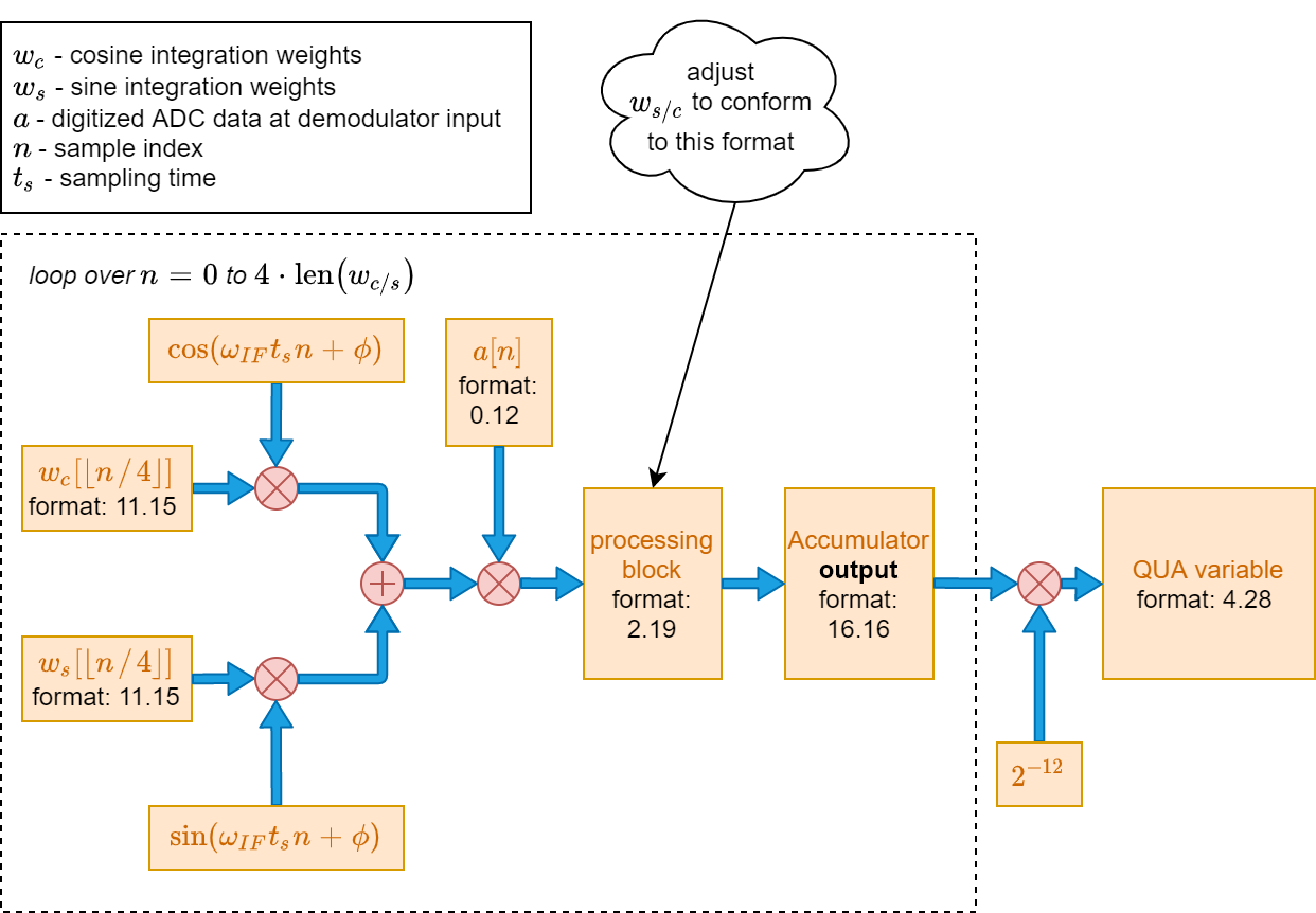
Fig. 1: Block diagram of demodulation operation in OPX. Numerical range corresponding to each fixed point format is given in the table below.
Warning
it is very important to make sure this section is well understood when using the demodulation operation, otherwise overflow may occur that will lead to corrupt results.
The simplest rule to remember to avoid overflow is as follows, valid when the demodulation is not very long: make sure the integration weights are such that when they multiply the raw ADC data, scaled to between -0.5 and 0.5, the result is between -2 and 2.
In Fig. 1 we see a breakdown of the demodulation operation in the equation above into steps, where the fixed point format in each step is shown. The translation from fixed point format to number ranges is given in the table below the figure. At each step, the input must be as shown to avoid overflow.
Note that the fixed point format of the integration weights is optimized to be compatible with the dynamic range of the ADC (12 bits), and the precision allows for very long demodulation sequences at the price of losing accuracy.
number format |
range of allowed values |
|---|---|
11.15 |
\([-1024:1024-\epsilon:\epsilon], \epsilon = 2^{-15} \simeq 3\cdot 10^{-5}\) |
0.12 |
\([-0.5:0.5-\epsilon:\epsilon], \epsilon = 2^{-12} \simeq 2.5\cdot 10^{-4}\) |
2.19 |
\([-2:2-\epsilon:\epsilon], \epsilon = 2^{-19} \simeq 2\cdot 10^{-6}\) |
16.16 |
\([-32768:32768-\epsilon:\epsilon], \epsilon = 2^{-16} \simeq 1.5\cdot 10^{-5}\) |
4.28 |
\([-8:8-\epsilon:\epsilon], \epsilon = 2^{-28} \simeq 4\cdot 10^{-9}\) |
Timing of the measurement operation
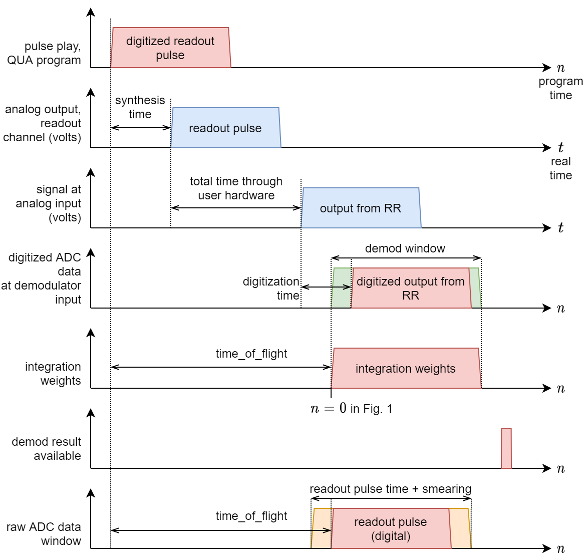
Fig.2: Timing diagram for the measurement operation
Warning
The phase of the readout pulse IF carrier is not necessarily equal to the phase of the IF tone used in the demodulation, and may also change between versions. Therefore the demodulation results may slightly change between versions.
So far we’ve discussed the demodulation operation in an isolated way. However, it occurs as a part of a measurement command that involves sending a pulse to the readout resonator, waiting some time, and then demodulating with the integration weights and possibly recording the raw ADC data. The parameters related to these timing operations are defined in the config, using the parameters:
time_of_flightsmearinglength of the readout pulse
length of integration weights
high values of the digital recording pulse
In the figure above we see how these parameters determine the timing of the measurement operation. Each waveform is represented schematically by a trapezoid. The red signals correspond to internal OPX signals, and the blue to actual analog waveforms. The relative timing of the operations is not to scale.
The green background in (d) corresponds to the window at which ADC data is taken and multiplied with the integration weights (see eq. (3)), and defines the \(n=0\) in that equation.
The yellow background in (g) corresponds to the additional window for ADC recording provided by the smearing parameter in the config.
We can see from the figure that the time_of_flight parameter has two uses: First, it determines the time from the beginning of the readout pulse and until the beginning
of the integration operation (d) and secondly, it sets the start of the ADC recording window, up to smearing, in (g).
It is also important to note that the demod window length is set solely by the length of the integration weights vector.
The length of the raw ADC data recodring window is set by the length of the readout pulse as well as the smearing parameter.