QUA Language Features
This document describes QUA language features that go beyond the simple use-case described in QUA overview section.
Measure statement features
The measure command is a central command in QUA. It allows for the acquisition of ADC data corresponding to a readout pulse, its storage and processing. The raw ADC data can be processed in several ways, as explained below.
Demodulation
where \(W^{4k+p}_{s,c}=\tilde{W}^{k}_{s,c} \forall p\in\{0,1,2,3\}\)
Types of demodulations:
Full demodulation
this is regular demodulation.
where \(n\) is the number of the total adc samples. The result is a fixed point value, with a format of 16.16. It must be manually right-shifted by 12 bits when loaded with QmJob.get_results().
Example:
The measure statement can be used in two ways:
measure([pulse], [element], [stream],
                ([integration_weights],[output_variable],[analog_output]),...)
Examples:
measure("readout", "RR", None, ("integW1",  I, "out1"))
measure("readout", "RR", None, ("integW1", I), ("integW1", Q))
measure([pulse], [element], [stream],
                demod.full([integration_weights],[output_variable],[analog_output]),...)
Examples:
measure("readout", "RR", None, demod.full("integW1", I, "out1"))
measure("readout", "RR", None, demod.full("integW1", I), demod.full("integW2", Q))
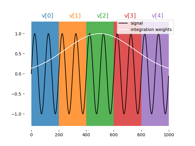
Sliced demodulation
The demodulation is sliced into chunks according to the formula below. Save the result in an array.
where \(C\) is the chunk size in units of 4 ns.
Illustrartion:
Syntax:
measure([pulse], [element], [stream],
                demod.sliced([integration_weights],[output_array],[chunk_size],[analog_output]),...)
Examples:
A = declare(fixed, size=10)
B = declare(fixed, size=4)
C = declare(fixed, size=4)
measure("readout", "RR", None, demod.sliced("integW1", A, 7, "out1"))
measure("readout", "RR", None,
                demod.sliced("integW2", A, 11), demod.sliced("integW3", A, 11))
Notes: A. chunk size is in units of 4ns. B. Currently, chunck size must be bigger or equal to 7 C. length of integration weights must be chunck_size * array_size
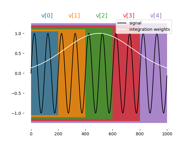
Accumulated demodulation
where \(C\) is the chunk size in units of 4 ns.
Illustration:
Syntax:
measure([pulse], [element], [stream], demod.accumulated([integration_weights],
                                                                                                                [output_array],
                                                                                                                [chunk_size],
                                                                                                                [analog_output]),...)
Examples:
A = declare(fixed, size=10)
B = declare(fixed, size=4)
C = declare(fixed, size=4)
measure("readout", "RR", None, demod.accumulated("integW1", A, 7, "out1"))
measure("readout", "RR", None,
                demod.accumulated("integW2", B, 11), demod.accumulated("integW3", C, 11))
Notes:
chunk size is in units of 4ns.
Currently, chunck’s size must be bigger or equal to 7
length of integration weights must be chunck_size * array_size
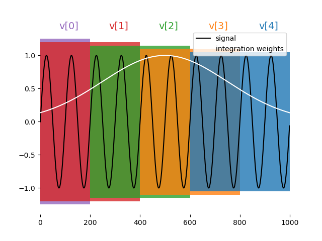
Moving window demodulation
where \(C\) is the chunk size in units of 4 ns and \(W\) is the chunks_per_window.
Illustration:
Syntax:
measure([pulse], [element], [stream], demod.moving_window([integration_weights],
                                                                                                                  [output_array],
                                                                                                                  [chunk_size],
                                                                                                                  [chunks_per_window],
                                                                                                                  [analog_output]),...)
Examples:
A = declare(fixed, size=10)
B = declare(fixed, size=4)
C = declare(fixed, size=4)
measure("readout", "RR", None, demod.moving_window("integW1", A, 7, 3, "out1"))
measure("readout", "RR", None,
                demod.moving_window("integW2", B, 5, 2), demod.moving_window("integW3", C, 5, 2))
Notes:
chunk size is in units of 4ns.
Currently, chunck size must be bigger or equal to 7
length of integration weights must be chunck_size * array_size
Chunk size must be less or equal to array_size
Integration
The same as demodulation but at zero frequency, namely:
where \(W^{4k+p}_{c}=\tilde{W}^{k}_{c} \forall p\in\{0,1,2,3\}\)
Types of integrations:
Full
syntax:
measure([pulse], [element], [stream],
                integration.full([integration_weights],[output_variable],[analog_output]),...)
Sliced
Syntax:
measure([pulse], [element], [stream],
                demod.integration([integration_weights],
                                                  [output_array],
                                                  [chunk_size],
                                                  [analog_output]),...)
Accumulated
Syntax:
measure([pulse], [element], [stream],
                integration.accumulated([integration_weights],
                                                                [output_array],
                                                                [chunk_size],
                                                                [analog_output]),...)
Moving window
Syntax:
measure([pulse], [element], [stream],
                integration.moving_window([integration_weights],
                                                                  [output_array],
                                                                  [chunk_size],
                                                                  [chunks_per_window],
                                                                  [analog_output]),...)
Time Tagging
The time-tagging feature populates a vector of time stamps, with 1 ns resolution, that are associated with voltage edges typically generated by a single photon counting module (SPCM). It is useful, for example, in quantum optics experiments for calculating the intesity cross correlation of multiple SPCMs.
configuring TT
A time-tag is generated when a voltage trigger edge is detected in the OPX analog input defined for the measurement quantum element. The trigger edge is defined according to a set of configuration parameters which can be added to the measuring quantum element. For example, in the configuration block below, the element qe1 has the time tagging parameters defined in the outputPulseParameters block.
'qe1': {
           "singleInput": {
               "port": (opx_one, 1)
           },
           'intermediate_frequency': IF_freq,
           'operations': {
               'measurement': 'readout_pulse'
           },
           "outputs": {
               'out1': [opx_one, 2]
           },
           'time_of_flight': TOF,
           'smearing': 0,
           'outputPulseParameters': {
                'signalThreshold': 200,
                'signalPolarity': 'Ascending',
                'derivativeThreshold': 100,
                'derivativePolarity': 'Ascending'
           }
       },
signalThreshold defines the threshold for detection in ADC units. signalPolarity defines whether is signal peak has a positive or negative voltage. It can be set to either Ascending or Descending (case sensitive). derivativeThreshold give the thereshold for the derivative in units of ACD/ns.
If these values are not specified, defaults are used. The user must supply eith all values, or none. The default values are as follows:
'outputPulseParameters': {
    'signalThreshold': 800,
    'signalPolarity': 'Descending',
    'derivativeThreshold': 300,
    'derivativePolarity': 'Descending'
    }
Using TT
Time-tagging is done in a meausre statment, with the following syntax:
measure([pulse], [element], [stream],time_tagging.raw([result_vec],[duration], [targetLen])
result_vec is a vector of integers that is populated by the measurement.
duration gives the maximum time window during which the statment waits for tag arrival. targetLen is an optional parameter which gives the number of tags which stops the measurment. The time-tagging operation ends either at the set duration or at the requested targetLen is acheived (first one of the two).
Sticky pulse
A quantum element can be defined as sticky by adding the hold_offset key to its configuration. Once defined in this way, it retains the final sample in its pulse, and any subsequent pulse will be referenced to that sample. A sticky element always ramps back to its DC offset value at the end of a program. This ramp can also be explicitly initiated by the ramp_to_zero function.
The sticky element behavior is simply shown in the following example. We first define the quantum element as follows:
"qe1": {
                        "singleInput": {
                                "port": ("con1", 1)
                        },
                        'intermediate_frequency':0,
                        'hold_offset':{'duration': 100},
                        'operations': {
                                'pulse': "pulse",
                        },

                }
Note the {‘duration’: 100} which sets the ramp to zero duration, in clock cycles. We also define a second quantum element qe2 which is not sticky.
We can then run a simple program playing the same constant pulse twice, for the two different quantum elements:
with program() as prog:
        play('pulse','qe1')
        wait(100,'qe1')
        play('pulse','qe1')
        wait(100,'qe2')
        play('pulse','qe2')
        wait(100,'qe2')
        play('pulse','qe2')
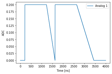
The resulting pulse sequence is shown below, where the sticky element is in blue and the non-sticky element is in oragne.
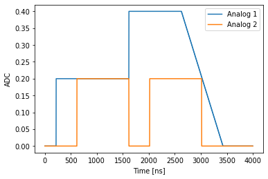
The duration of each pulse is 1000 clock cycles, nevertheless the blue pulse maintains its final value between its first and second occurance. Furthermore, the second occurance of the pulse to the sticky qe1 element is referenced to the last pulse sample. At the end of the program, the blue trace rampd to zero within 100 clock cycles, as defined in the configuration.
Voltage easing
A ramp to zero can be initiated on a sticky pulse at any point by calling the ramp_to_zero(qe,duration) function. The duration parameter is optional and can be used to override the configuration value. The waveform below was generated by running this program: .. code-block:: python
- with program() as prog:
play(‘pulse’,’qe1’) ramp_to_zero(‘qe1’,100) play(‘pulse’,’qe1’)
Note the first pulse eases to zero at a double rate compared to the second one.
Ramp pulse
It’s possible to generate a voltage ramp by using the ramp(slope) command. The slope argunment is specified in units of V/ns. Usage of this feature is as follows:
play(ramp(0.0001),'qe1',duration=1000)
Note
pulse duration must be specified if the ramp feature is used
The slope can either be a literal (as shown above) or a QUA variable or expression. For example, consider the following snippet.
d=1000
max_v=0.35
n=1000
with program() as myFirstProgram:
        a = declare(fixed)
        with for_(a, max_v/d/10, a <= max_v/d, a +max_v/d/n):
                play(ramp(a/2), 'qe1', duration=d)
                play(ramp(-a/2), 'qe1', duration=d)
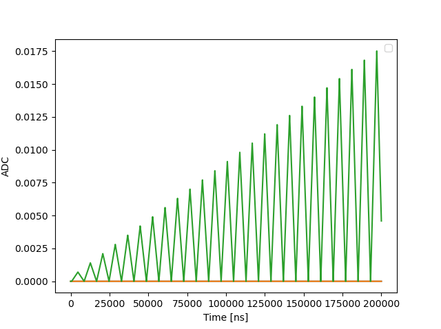
The quantum element qe1 is defined as a sticky pulse and the resulting waveform is therefore triangular in each loop step as is shown in the image below.
External triggering
res.my_stream.has_data_loss()
OPX operations like play and measure can be condition upon a rising edge from the external trigger.
This is defined by the following command:
wait_for_trigger(element, pulse_to_play=None):
For example, if we want to play to qe1 after a trigger input, we can write:
    wait_for_trigger('qe1', 'wait_pulse')
play('qe1_pulse','qe1')
then ‘wait_pulse’ is played at the output of ‘qe1’ until the trigger is received and the ‘qe1_pulse’ is then played.
Warning
The maximum allowed voltage value for the digital trigger is 1.8V. A voltage higher than this can damage the controller.
Frequency chirp
This feature allows to perform a linear sweep of the element’s intermediate frequency in time. Chirp parameters can be updated in run-time, inside a QUA program.
Basic usage of this feature is performed as follows:
play('pulse', 'qe', chirp=(rate, units))
Becuase the supported chirp rate spans many orders of magnitude, from mHz/sec to GHz/sec, it is defined by both a rate numeric variable and a units string. Supported units are (exactly) one of the following: ‘Hz/nsec’,’mHz/nsec’,’uHz/nsec’,’pHz/nsec’ or their equivalent rates per-second: ‘GHz/sec’,’MHz/sec’,’KHz/sec’,’Hz/sec’,’mHz/sec’. The rate itself is an integer, which can either be a QUA variable or a python literal.
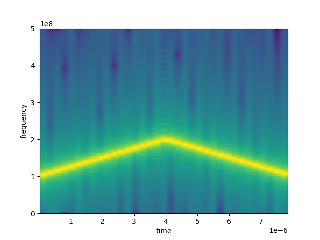
A spectrogram of a positive chirp rate followed by a negative rate is shown below. The chirp duration is defined by the duration of the used pulse.
with program() as prog:
        chirp_rate = declare(int, value=25000)
        play("pulse", "qe", chirp=(chirp_rate , 'Hz/nsec'))
        play("pulse", "qe", chirp=(-25000, 'Hz/nsec'))
Note
The duration keyword for dynamically stretching a pulse cannot be used in conjunction with a chirp
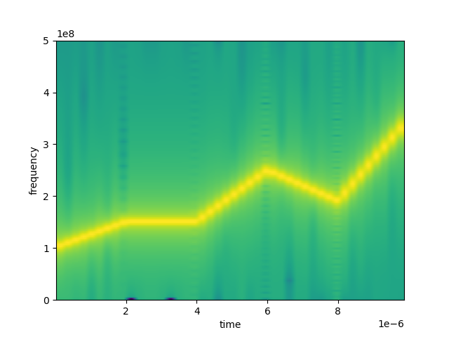
It is possible to directly define a piecewise linear chirp by providing a list of rates as shown below. This is a convenient method to approximate non-linear chirp rates.
with program() as prog:
        a = declare(int, value=[25000, 0, 50000, -30000, 80000])
        play("pulse", "qe", chirp=(a, 'Hz/nsec'))

# equivalent program:
with program() as prog:
        play("pulse", "qe", chirp=([25000, 0, 50000, -30000, 80000], 'Hz/nsec'))
The hardware implementation of the chirp updates the frequency as following:
Note that this discrete implementation of the chirp differs by one time-step (clock cycle) from the continuous frequency chirp which yields
Pulse Memory Compression
In order to optimize memory allocation the QUA compiler takes into account the freuency content of each pulse. Each waveform’s FFT is used to calculate the cutoff frequency f_cut under which 99.9% of the waveform’s energy lies. Each waveform then receives a score based on his cutoff frequency f_cut and the waveform’s length. The memory is then allocated to each waveform based on this score. The compiler also calculates the error between the original and interpolated waveforms and issues an error if it is larger than 1e-4:
ERROR - Insufficient memory for waveform wf_long. Maximum allowed compression error is 0.0001 but got error of 0.006166048912738864.
The user can add to the waveform the parameter maxAllowedError:
% Setting the 'maxAllowedError' parameter to 1e-2 instead of the default 1e-3
'waveforms': {
        'wf1': {
        'type': 'arbitrary',
        'samples': [0.49, 0.47, 0.44, ...],
        'maxAllowedError': 1e-2
        },
That will override the default value (1e-4) allowing the user to tweak memory allocation. Alternatively, the user can simply control the sampling ratio of the pulse:
% Setting the 'maxAllowedError' parameter to 1e-2 instead of the default 1e-3
'waveforms': {
        'wf1': {
        'type': 'arbitrary',
        'samples': [0.49, 0.47, 0.44, ...],
        'sampling_rate': 0.5
        },
The ‘sampling_rate’ parameter specifies the sampling rate, a number between 0 and 1 with units of GS/sec (giga-samples per second).
Any time a pulse is compressed, the compiler will output a warning and the compression factor:
WARNING - Waveform wf_long was compressed with rate 0.6548853220189729 and error of 1.6128764990241962E-13
Dynamic pulse duration
The duration of the pulse can stretched (but, in the case of an arbitrary waveform, not compressed) using the “duration” parameter:
# Stretching the pulse length
play(pulse, element, duration = 100)
# One can also use a variable or an expression
play(pulse, element, duration = 2*t+100)
The stretched pulse is calculated from the original pulse using a 3rd order Lagrange interpolator on a 4 points running window. The duration parameter can accept a general mathematical expression composed of operators (+, -, *, /), numbers, QUA variables and QUA functions (such as cos and sin).
Warning
when playing an arbitrary waveform, if the value of the duration parameter is set to below the original pulse length, corrupted output may occur.
Warning
The interpolation mechanism used to create dynamically stretched waveform will add a latency of 0.5nsec with respect to the position in time of the original waveform.